Tutorial on using blotter
This tutorial provides some simple use cases for blotter. To start with,
import the library and create a Blotter() object
In [1]: from blotter import blotter

In [2]: import pandas as pd

In [3]: import numpy as np

In [4]: import matplotlib.pyplot as plt

In [5]: pd.options.display.max_rows = 10

In [6]: blt = blotter.Blotter(
   ...:            prices="data/prices",
   ...:            interest_rates="data/daily_interest_rates.csv",
   ...:            accrual_time=pd.Timedelta(16, unit="h"),
   ...:            eod_time=pd.Timedelta(16, unit="h"),
   ...:            sweep_time=pd.Timedelta(16, unit="h"),
   ...:            base_ccy="USD",
   ...:            margin_charge=0.015
   ...:           )
   ...:

In [7]: blt.connect_market_data()
In the above we provide a path to a folder of csv files for the prices of the
instruments we intend to trade as well as a file containing interest rates
for each of the currencies transacted in. The accrual_time corresponds to
the time of day which interest and margin are accrued. The interest rates
provided must include an entry for this time of day. eod_time is the time
at which daily PnL is calculated. The csv files of prices provided must
included a price for this time of day for each day when an instrument has an
open position excluding weekends. Note that this includes market holidays where
there may be no trading, thus the user is responsible for appropriately filling
the data. sweep_time defines the time of day when closed PnL in
currencies other than the base currency are repatriated to the base currency.
Daily FX rates corresponding to the sweep_time must be provided in the csv
files of prices for each currency in the non base currency, used for conversion
to the base.
Now we define the meta data for the instruments we plan to trade.
In [8]: blt.define_generic("AUDUSD", ccy="USD", margin=0, multiplier=1,
   ...:                        commission=2.5, isFX=True)
   ...:

In [9]: blt.define_generic("USDJPY", ccy="JPY", margin=0, multiplier=1,
   ...:                        commission=2.5, isFX=True)
   ...:

In [10]: blt.map_instrument(generic="AUDUSD", instrument="AUDUSD")

In [11]: blt.map_instrument("USDJPY", "USDJPY")

In [12]: blt.define_generic("CL", ccy="USD", margin=0.1, multiplier=1000,
   ....:                       commission=2.5, isFX=False)
   ....:

In [13]: blt.map_instrument("CL", "CLZ2008")
We use a vary simple trading strategy which buys and holds Crude and which uses 5 day momentum for deciding whether to buy or sell AUDUSD and USDJPY. For simplicity, we will also trade at the 4:00 P.M. and use the same prices as used internally in the Blotter.
In [14]: crude = pd.read_csv("data/prices/CLZ2008.csv", parse_dates=True, index_col=0)

In [15]: aud = pd.read_csv("data/prices/AUDUSD.csv", parse_dates=True, index_col=0)

In [16]: jpy = pd.read_csv("data/prices/USDJPY.csv", parse_dates=True, index_col=0)
In [17]: timestamps = pd.date_range("2008-01-02", "2008-05-27", freq="b")
In [18]: timestamps = timestamps + pd.Timedelta("16h")
In [19]: timestamps = (timestamps.intersection(crude.index)
....: .intersection(aud.index).intersection(jpy.index))
....:
In [20]: ts = timestamps[0]
In [21]: blt.trade(ts, "CLZ2008", 10, float(crude.loc[ts]))
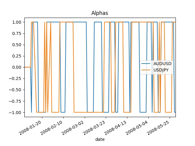
In [22]: aud_alpha = np.sign(np.log(aud / aud.shift(5))).fillna(value=0)
In [23]: jpy_alpha = np.sign(np.log(jpy / jpy.shift(5))).fillna(value=0)
In [24]: signal = pd.concat([aud_alpha, jpy_alpha], axis=1)
In [25]: signal.columns = ["AUDUSD", "USDJPY"]
In [26]: signal.plot(title="Alphas")
Out[26]: <matplotlib.axes._subplots.AxesSubplot at 0x7fadfe3dc4e0>
In [27]: def calc_trade(position, alpha):
   ....:     if position.empty:
   ....:         return alpha
   ....:     else:
   ....:         return alpha*1000000 - position
   ....:
In [28]: for ts in timestamps:
   ....:     pos = blt.get_instruments()
   ....:     pos = pos.drop("CLZ2008")
   ....:     trds = calc_trade(pos, signal.loc[ts,:])
   ....:     aud_qty = float(trds.loc["AUDUSD"])
   ....:     aud_price = float(aud.loc[ts])
   ....:     jpy_qty = float(trds.loc["USDJPY"])
   ....:     jpy_price = float(jpy.loc[ts])
   ....:     blt.trade(ts, "AUDUSD", aud_qty, aud_price)
   ....:     blt.trade(ts, "USDJPY", jpy_qty, jpy_price)
   ....:
If at any given time we want to get the current holdings for each instrument in units of the instrument we can obtain these using
In [29]: blt.get_instruments()
Out[29]:
AUDUSD     1000000.0
CLZ2008         10.0
USDJPY     1000000.0
dtype: float64
If we want to get the value of the current holindgs denominated in the base currency, we can use
In [30]: ts = pd.Timestamp("2008-05-28T16:00:00")

In [31]: blt.get_holdings_value(ts)
Out[31]:
AUDUSD      962600.0
CLZ2008    1299600.0
USDJPY     1000000.0
dtype: float64
Note that in the call above we need to provide a timestamp since we are doing an FX conversion under the hood. Finally we will close out all our positions and calculate our closed PnL.
In [32]: prices = {"AUDUSD": aud, "USDJPY": jpy, "CLZ2008": crude}

In [33]: instrs = blt.get_instruments()

In [34]: for instr, qty in instrs.iteritems():
   ....:     price = float(prices[instr].loc[ts])
   ....:     blt.trade(ts, instr, -qty, price)
   ....:
If we want to look at a full history of positions we can use
In [35]: blt.get_holdings_history()
Out[35]:
{'JPY': {'USDJPY': 2008-01-09 16:00:00          1.0
  2008-01-10 16:00:00    1000000.0
  2008-01-14 16:00:00   -1000000.0
  2008-01-22 16:00:00    1000000.0
  2008-01-23 16:00:00   -1000000.0
                           ...
  2008-05-15 16:00:00   -1000000.0
  2008-05-16 16:00:00    1000000.0
  2008-05-20 16:00:00   -1000000.0
  2008-05-27 16:00:00    1000000.0
  2008-05-28 16:00:00          0.0
  dtype: float64}, 'USD': {'AUDUSD': 2008-01-09 16:00:00         -1.0
  2008-01-10 16:00:00    1000000.0
  2008-01-16 16:00:00   -1000000.0
  2008-01-24 16:00:00    1000000.0
  2008-02-07 16:00:00   -1000000.0
                           ...
  2008-05-07 16:00:00   -1000000.0
  2008-05-08 16:00:00    1000000.0
  2008-05-13 16:00:00   -1000000.0
  2008-05-16 16:00:00    1000000.0
  2008-05-28 16:00:00          0.0
  dtype: float64, 'CLZ2008': 2008-01-02 16:00:00    10000.0
  2008-05-28 16:00:00        0.0
  dtype: float64}}
Lastly we calculate all automatic events (interest charges, PnL sweeps and margin charges).
In [36]: ts = pd.Timestamp("2008-05-29T16:00:00")

In [37]: blt.automatic_events(ts)
Get holdings intraday, show errors when getting holdings without prices Show event log of trades
In [38]: pnls = blt.get_pnl_history()
In [39]: pnls
Out[39]:
{'AUD': pnl closed pnl open pnl
2008-01-10 16:00:00 0.0 0.0 0
2008-01-11 16:00:00 0.0 0.0 0
2008-01-14 16:00:00 0.0 0.0 0
2008-01-15 16:00:00 0.0 0.0 0
2008-01-16 16:00:00 0.0 0.0 0
... ... ... ...
2008-05-22 16:00:00 0.0 0.0 0
2008-05-23 16:00:00 0.0 0.0 0
2008-05-26 16:00:00 0.0 0.0 0
2008-05-27 16:00:00 0.0 0.0 0
2008-05-28 16:00:00 0.0 0.0 0
[100 rows x 3 columns],
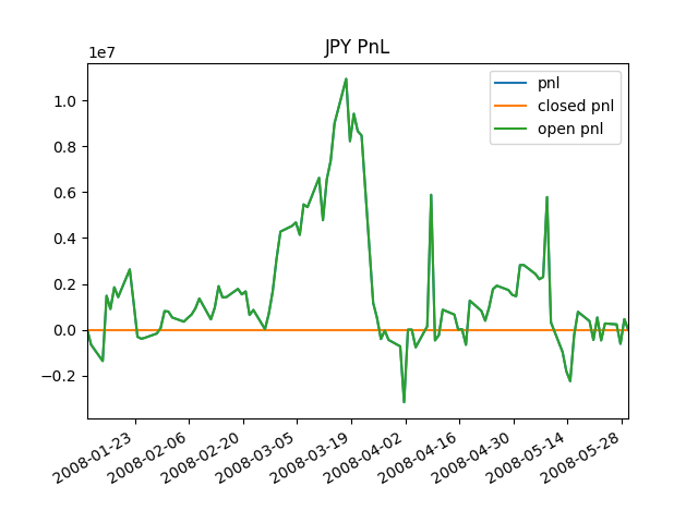
'JPY': pnl closed pnl open pnl
2008-01-10 16:00:00 -2.600000e-01 -5.128276e-17 -0.26
2008-01-11 16:00:00 -6.600003e+05 0.000000e+00 -660000.26
2008-01-14 16:00:00 -1.370000e+06 0.000000e+00 -1370000.26
2008-01-15 16:00:00 1.480000e+06 -9.640644e-11 1480000.00
2008-01-16 16:00:00 9.000000e+05 1.039098e-10 900000.00
... ... ... ...
2008-05-23 16:00:00 2.700000e+05 1.946319e-10 270000.00
2008-05-26 16:00:00 2.300000e+05 -1.909939e-11 230000.00
2008-05-27 16:00:00 -6.200000e+05 2.091838e-10 -620000.00
2008-05-28 16:00:00 4.600000e+05 -2.046363e-10 460000.00
2008-05-29 16:00:00 -3.819878e-11 -3.819878e-11 0.00
[101 rows x 3 columns],
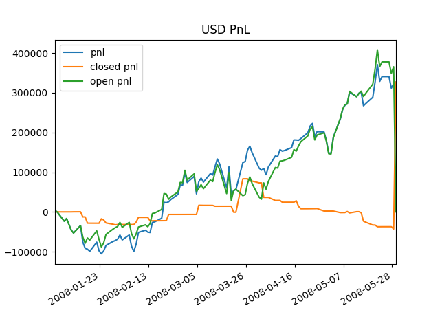
'USD': pnl closed pnl open pnl
2008-01-03 16:00:00 3703.575992 3.575992 3700.0
2008-01-04 16:00:00 -378.362498 21.637502 -400.0
2008-01-07 16:00:00 -23472.424107 27.575893 -23500.0
2008-01-08 16:00:00 -16566.416225 33.583775 -16600.0
2008-01-09 16:00:00 -31360.502841 39.497159 -31400.0
... ... ... ...
2008-05-23 16:00:00 340893.954279 -37206.045721 378100.0
2008-05-26 16:00:00 340809.446406 -37190.553594 378000.0
2008-05-27 16:00:00 311825.158817 -37174.841183 349000.0
2008-05-28 16:00:00 322668.346880 -43031.653120 365700.0
2008-05-29 16:00:00 327022.413244 327022.413244 0.0
[106 rows x 3 columns]}
In [40]: pnls["USD"].plot(title="USD PnL")
����������������������������������������������������������������������������������������������������������������������������������������������������������������������������������������������������������������������������������������������������������������������������������������������������������������������������������������������������������������������������������������������������������������������������������������������������������������������������������������������������������������������������������������������������������������������������������������������������������������������������������������������������������������������������������������������������������������������������������������������������������������������������������������������������������������������������������������������������������������������������������������������������������������������������������������������������������������������������������������������������������������������������������������������������������������������������������������������������������������������������������������������������������������������������������������������������������������������������������������������������������������������������������������������������������������������������������������������������������������������������������������������������������������������������������������������������������������������������������������������������������������������������������������������������������������������������������������������������������������������������������������������������������������������������������������������������������������������������������������������������������������������������������������������������������������������������������������������������������������������������������������������������������������������������������������������������������������������������������������������������������������������������������������������������������������������������������������������������������������������������������������������������������������������������������������������������������������������������������������Out[40]: <matplotlib.axes._subplots.AxesSubplot at 0x7fadfe6f5be0>
In [41]: pnls["JPY"].plot(title="JPY PnL")
Out[41]: <matplotlib.axes._subplots.AxesSubplot at 0x7fadfe678b00>
Another helpful thing can be looking at the blotter event log, which contains a record of all actions performed by the Blotter object on its instance of Holdings.
In [42]: blt.event_log[-10:]
Out[42]:
['CASH|{"timestamp": "2008-05-28 16:00:00", "ccy": "USD", "quantity": 962600.0}',
 'CASH|{"timestamp": "2008-05-28 16:00:00", "ccy": "AUD", "quantity": -1000000.0}',
 'TRADE|{"timestamp": "2008-05-28 16:00:00", "ccy": "USD", "commission": 2.5, "instrument": "CLZ2008", "price": 129.96, "quantity": -10000.0}',
 'TRADE|{"timestamp": "2008-05-28 16:00:00", "ccy": "JPY", "commission": 2.5, "instrument": "USDJPY", "price": 104.65, "quantity": -1000000.0}',
 'CASH|{"timestamp": "2008-05-28 16:00:00", "ccy": "JPY", "quantity": 104650000.0}',
 'CASH|{"timestamp": "2008-05-28 16:00:00", "ccy": "USD", "quantity": -1000000.0}',
 'INTEREST|{"timestamp": "2008-05-29 16:00:00", "ccy": "JPY", "quantity": -8.538355345205462}',
 'INTEREST|{"timestamp": "2008-05-29 16:00:00", "ccy": "USD", "quantity": -1.4318978007000005}',
 'PNL|{"timestamp": "2008-05-29 16:00:00", "prices": {}}',
 'PNL_SWEEP|{"timestamp": "2008-05-29 16:00:00", "ccy1": "JPY", "ccy2": "USD", "quantity1": -459988.96164466254, "quantity2": 4360.498261869964}']